Wire Frames, Partial Derivatives, and Tangent Planes

Section 6.2 Wire Frames, Partial Derivatives, and Tangent Planes

Link to worksheets used in this section ¹

A standard technique in mathematics courses is to try to break a complicated problem into smaller and easier problems. For functions of several variables this can be done by looking at the variables one at a time, and treating the other variables as constants. Then we are back to considering functions of a single variable.

Subsection 6.2.1 Wire frames

We start by returning to Example 6.1.12 from Section 6.1, and seeing what information can be obtained by looking at one variable at a time.

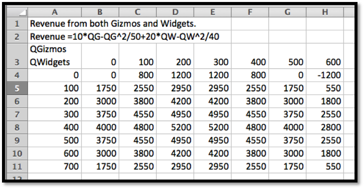
Example 6.2.1. Optimizing Revenue with Two Products.

Figure 6.2.2. Video presentation this example

I have a company that produces two products, widgets and gizmos. The two demand functions are:

\begin{align*} \PriceGizmo\amp =10-\frac{\QuantityGizmo}{50}=10-\frac{\text{QG}}{50}\\ \PriceWidget\amp =20-\frac{\QuantityWidget}{40}=20-\frac{\text{QW}}{40}\text{.} \end{align*}

This gives me the following revenue function:

\begin{equation*} \revenue(\QG,\QW)=10QG-\frac{\QG^2}{50}+20\QW-\frac{\QW^2}{40}\text{.} \end{equation*}

Look at the functions of one variable obtained by treating either QG or QW as a constant. Use this information to find where we maximize revenue.

Solution.

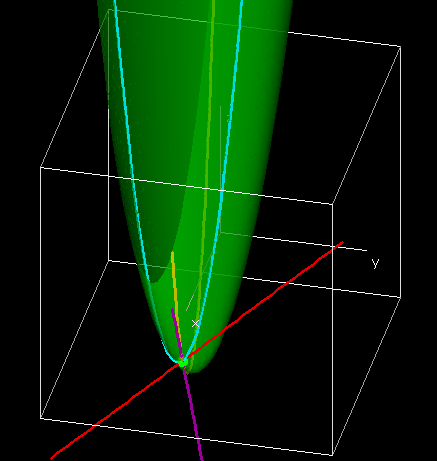
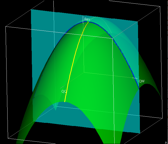
In terms of the last example, we want to start with a table and a wire frame chart.

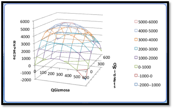
The wires are obtained by intersecting the graph of the function with a plane where QW or QG is held constant.

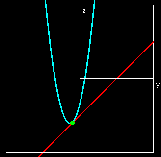
Thus, when we treat either QW or QG as a constant we effectively are looking at one of the wires of the wire frame. To illustrate this, we will look at the wires corresponding to $\QW=400$ and $\QG=300\text{.}$ When $\QG=300\text{,}$ our revenue function simplifies to

\begin{align*} \revenue(300,\QW) \amp =3000-1800+20\text{QW}-\frac{\text{QW}^2}{40}\\ \amp =1200+20\QW-\frac{\QW^2}{40}\text{.} \end{align*}

Thus, the wire corresponding to $\QG=300$ is a parabola that bends down.

The interactive below shows how the wireframe is built from cuves defined by slice curves defined by cut planes.

Figure 6.2.3. Wire mesh

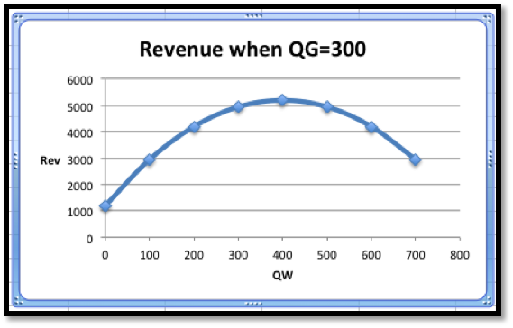
To find the vertex of the parabola, we take the derivative of our function of QW and set it equal to zero.

\begin{equation*} \frac{d}{d\QW} \revenue(300,\QW)=20-\frac{\QW}{20}\text{.} \end{equation*}

This derivative is zero when $\QW=400\text{.}$ That is the only possible place on this wire where we can have a maximum.

Similarly, when $\QW=400\text{,}$

\begin{align*} \revenue(\QG,400) \amp =10\QG-\frac{\QG^2}{50}+4000\\ \frac{d}{d\QG} \revenue(\QG,400)\amp =10-\frac{\QG}{25}\text{.} \end{align*}

This derivative is zero when $\QG=250\text{.}$ That is the only possible place on this wire where we can have a maximum.

Putting the information together, the maximum must occur at $(250,400)\text{.}$ Putting these values back in the original equation gives a maximum of $5250 for the revenue function.

Subsection 6.2.2 Partial Derivatives

The procedure we used in the first example of replacing one variable with a constant and then taking the derivative of the resulting single variable function is a bit cumbersome. We can simplify the process by taking the derivative of the original function with respect to one variable while treating the other variables as constants. This is referred to as taking a partial derivative. There is also a change in notation. The familiar derivative of $f$ with respect to $x$ uses the symbol $\frac{d}{dx} f\text{,}$ while the partial derivative with respect to $x$ uses the symbol $\frac{\partial }{\partial x} f\text{,}$ or $f_x\text{.}$ Similarly, the partial derivative with respect to $y$ uses the symbol$\frac{\partial }{\partial y} f\text{,}$ or $f_y\text{.}$

Example 6.2.4. Finding and Interpreting Partial Derivatives.

Find the partial derivatives of $f(x,y)=x^2+ 2xy+3y^2-4x-3y$ at $(x,y)=(3.5,-0.5)\text{.}$ Explain what the partial derivatives mean in terms of the graph.

Solution.

It is useful to look at a picture with the graph, the two curves obtained by keeping $x=3.5$ and $y=1.5\text{,}$ and the tangent lines to those curves.

We also want to look at the slices corresponding keeping $x=-3.5$ and $y=.5\text{.}$

The yellow curve is obtained by fixing $y$ and letting $x$ vary. The blue curve is obtained by fixing $y$ and letting $x$ vary. We now take the partial derivatives with respect to both variables.

\begin{align*} \frac{\partial }{\partial x} f(x,y)\amp =2x+ 2y+0-4-0=2x+2y-4\\ \frac{\partial }{\partial x} f(3.5,-0.5)\amp =7- 1-4=2\\ \frac{\partial }{\partial y} f(x,y)\amp =0+2x+6y+0-3=2x+6y-3\\ \frac{\partial }{\partial y} f(3.5,-0.5)\amp =7-3-3=1\text{.} \end{align*}

The partial derivatives give the slopes of the purple and red lines above. At the point $(3.5,-0.5)\text{,}$ the (yellow) curves obtained by treating y as a constant and letting $x$ vary has a (magenta) tangent line with a slope of $2\text{,}$ the value $\frac{\partial }{\partial x} f(3.5,-0.5)\text{.}$ At the point $(3.5,-0.5)\text{,}$ the (blue) curves obtained by treating $x$ as a constant and letting $y$ vary has a (red) tangent line with a slope of 1, the value $\frac{\partial }{\partial y} f(3.5,-0.5)\text{.}$

Subsection 6.2.3 Tangent Planes and Linear Approximation

For functions of one variable, we had two main uses of the derivative. One was to identify candidate points for maxima and minima. We will look at critical points and extrema in the next section. The other use of the derivative was to produce a linear approximation or tangent line. We can generalize the tangent line for one variable to a tangent plane for two variables. For a function $f(x)\text{,}$ we used the value of the point, $(x_0,f(x_0))$ and the slope $f(x_0)$ to get the equation of the tangent line approximation near $x_0\text{.}$

Tangent line.

\begin{equation*} \text{Linear }f(x)=f' (x_0 )(x-x_0 )+f(x_0 )\text{.} \end{equation*}

For a function, $f(x,y)\text{,}$ of two variables, we simply use partials for the slopes.

Tangent Plane.

\begin{equation*} \text{Linear }f(x ,y)=f_x (x_0,y_0 )(x-x_0 )+f_y (x_0,y_0 )(y-y_0)+f(x_0,y_0 )\text{.} \end{equation*}

Example 6.2.5. Approximating with a Tangent Plane.

The general Cobb-Douglas production function determines the Production (P), in terms of the variables Labor (L) and Capital (C):

\begin{equation*} \text{Production(Labor,Capital)}=c \text{Labor}^{\alpha} \text{Capital}^{\beta}\text{,} \end{equation*}

or using short-hand notation:

\begin{equation*} P(L,C)=c L^{\alpha} C^\beta\text{,} \end{equation*}

where $c\text{,}$ $\alpha\text{,}$ and $\beta$ are constants. For our widget factory, this becomes

\begin{equation*} \text{Production(Labor,Capital)}=10 L^{0.75} C^{0.25}\text{,} \end{equation*}

with labor production and capital in the appropriate units.

Find $\Production(81,16)\text{.}$ Use a linear approximation to estimate $\Production(85,14)\text{.}$

Solution.

We answer the first question by substituting the values into the equation.

\begin{equation*} \Production(81,16)=10*81^{0.75}*16^{0.25}=10*27*2=540\text{.} \end{equation*}

To produce the tangent plane we take the partial derivatives and evaluate them at our base point.

\begin{align*} \Production_{\Labor} (\Labor,\Capital)\amp =10*.75 \Labor^{-0.25} \Capital^{0.25}\\ \Production_{\Labor} (81,16)\amp =10*.75 (1/3) *2=5\\ \Production_{\Capital} (\Labor,\Capital)\amp =10*{0.25} \Labor^{0.75 } \Capital^{-0.75}\\ \Production_{\Capital} (81,16)\amp =10*.25 *27 (1/8)=8.4375\text{.} \end{align*}

This gives us our tangent plane:

\begin{equation*} \Production(\Labor,\Capital)\approx 5(\Labor-81)+8.4375(\Capital-16)+540\text{.} \end{equation*}

Substituting in values gives our estimate.

\begin{equation*} \Production(85,14)\approx 5(85-81)+8.4375(14-16)+540=543.125\text{.} \end{equation*}

In the case of the last example, evaluating the linear approximation was nicer than evaluating the function directly because the 4th roots of 16 and 81 are whole numbers, while the 4th roots of 85 and 14 are harder to compute. For real world functions, evaluating functions may involve a substantial investment of time and money, depending on the nature of the function.

Linear Approximations of Functions of More than Two Variables.

In this section we have focused on functions of 2 variables since their graphs are surfaces in 3 dimensions, which is a familiar concept. For real world functions, we are often concerned with functions of many variables. The concept of partial derivative easily extends, with one variable and multiple parameters. Finding the linear approximation also extends without difficulty. We simply have a linear term for each variable.

Reading Questions 6.2.4 Reading Check

1. Reading check, Wire Frames, Partial Derivatives, and Tangent Planes.

This question checks your reading comprehension of the material is section 6.2, Wire Frames, Partial Derivatives, and Tangent Planes, of Business Calculus with Excel. Based on your reading, select all statements that are correct. There may be more than one correct answer. The statements may appear in what seems to be a random order.

Partial derivatives are not defined for functions of three variables.
The partial derivative of $f$ with respect to $x$ is represented as $\frac{\partial}{\partial x} f\text{.}$
A partial derivative is obtained by treating all but one variable as a constant.
A tangent plane can be used for a linear approximation of a function of two variables.
Partial derivatives give the slope of the tangent line for the curve obtained by holding one variable constant.
The partial derivative of $f$ with respect to $x$ is represented as $f_x\text{.}$
We cannot graph functions of two variables.
None of the above

Exercises 6.2.5 Exercises: Wire Frames, Partial Derivatives, and Tangent Planes Problems

Exercise Group.

For the given functions and points $P_1$ and $P_2\text{:}$

Give the 2 functions of one variable through $P_1$ obtained by holding each variable constant.
Find the partial derivatives of the original function.
Evaluate the partial derivatives at $P_1\text{.}$
Give the equation of the tangent plane through $P_1\text{.}$
The approximation at $P_2$ obtained from the tangent plane.

1.

The function is $f(x,y)=x^2+3xy+4y^2\text{,}$ $P_1=(4,2)\text{,}$ and $P_2=(3,2.5)\text{.}$

Solution.

Give the 2 functions of one variable through $P_1$ obtained by holding each variable constant.

\begin{align*} f(4,y)\amp =16+12y+4y^2\\ f(x,2)\amp =x^2+6x+16\text{.} \end{align*}
Find the partial derivatives of the original function.

\begin{align*} f_x (x,y) \amp = 2x+3y\\ f_y (x,y) \amp = 3x+8y\text{.} \end{align*}
Evaluate the partial derivatives at $P_1\text{.}$

\begin{align*} f_x (4,2) \amp = 8+6=14\\ f_y (4,2) \amp = 12+16=28\text{.} \end{align*}
Give the equation of the tangent plane through $P_1\text{.}$

We need $f(4,2)=16+24+16=56$ for the equation of the tangent plane.

\begin{align*} \Linear f(x ,y) \amp = f_x (x_0,y_0 )(x-x_0 )+f_y (x_0,y_0 )(y-y_0 )+f(x_0,y_0 )\\ \Linear f(x,y) \amp = 14(x-4)+28(y-2)+56\text{.} \end{align*}
The approximation at $P_2$ obtained from the tangent plane.

\begin{align*} \Linear f(3,2.5) \amp = 14(3-4)+28(2.5-2)+56\\ \amp = -14+14+56=56\text{.} \end{align*}

2.

The function is $f(x,y)=(x+3y)/(x^2+y^2 )\text{,}$ $P_1=(2,3)\text{,}$ and $P_2=(3,2.5)\text{.}$

3.

The function is $f(x,y)=(x^2)(x+2^y)\text{,}$ $P_1=(3,-1)\text{,}$ and $P_2=(3,0)\text{.}$

Solution.

Give the 2 functions of one variable through $P_1$ obtained by holding each variable constant.

\begin{align*} f(3,y) \amp = 9(3+2^y)\\ f(x,-1) \amp = (x^2 )(x+2^{-1} )= x^3+\frac{1}{2} x^2\text{.} \end{align*}
Find the partial derivatives of the original function.

\begin{align*} f_x (x,y) \amp = (2x)(x+2^y )+(x^2 )(1+0 ) \text{ (product rule)}\\ \amp = 2x^2+2x 2^y+x^2=3x^2+(2x)2^y\\ f_y (x,y) \amp = \frac{\partial}{\partial y} (x^2 )(x+2^y ) \quad (\text{ Take partial derivative wrt }y)\\ \amp = \frac{\partial}{\partial y}(x^3+x^2 2^y ) \qquad\text{ (Simplify the expression)}\\ \amp = x^2 2^y \ln(2) \qquad (x \text{ is treated as a constant so the }x^3\text{ term drops out)}\text{.} \end{align*}
Evaluate the partial derivatives at $P_1\text{.}$

\begin{align*} f_x (3,-1) \amp = 27+(6) 2^{-1}=27+3=30\\ f_y (3,-1) \amp = 9*\frac{1}{2} \ln(2)=\frac{9}{2} \ln(2)\text{.} \end{align*}
Give the equation of the tangent plane through $P_1\text{.}$

We need $f(3,-1)=9*\frac{7}{2}=\frac{63}{2}$ for the equation of the tangent plane

\begin{align*} \Linear f(x ,y) \amp = f_x (x_0,y_0 )(x-x_0 )+f_y (x_0,y_0 )(y-y_0 )+f(x_0,y_0 )\\ \Linear f(x ,y) \amp = 30 (x-3)+\frac{9}{2} \ln(2) (y+1)+\frac{63}{2}\text{.} \end{align*}
The approximation at $P_2$ obtained from the tangent plane.

\begin{equation*} \Linear f(3,0)=30* (0)+\frac{9}{2} \ln(2) *(1)+\frac{63}{2}=\frac{9}{2} \ln(2)+\frac{63}{2}\text{.} \end{equation*}

4.

The function is the revenue function for selling widgets and gizmos with demand price functions

\begin{align*} \PriceGizmo \amp = 30-\frac{\QuantityGizmo}{50}-\frac{\QuantityWidget}{300}\\ \PriceWidget \amp = 20-\frac{\QuantityWidget}{40}-\frac{\QuantityGizmo}{500}\text{,} \end{align*}

and $P_1=(\QuantityGizmo,\QuantityWidget)=(1000,500)\text{,}$ and $P_2=(1050,575)\text{.}$

5.

The function is the revenue function for selling widgets and gizmos with demand price functions

\begin{align*} \PriceGizmo \amp = 30(0.95)^{(\QuantityGizmo/100)}-\frac{\QuantityWidget}{300}\\ \PriceWidget \amp = 20(0.9)^{(\QuantityWidget/150)}-\frac{\QuantityGizmo}{250}\text{,} \end{align*}

and $P_1=(\QuantityGizmo,\QuantityWidget)=(800,400)\text{,}$ and $P_2=(750,425)\text{.}$

Solution.

For the sake of notation we will use the following abbreviations:

\begin{align*} \PG \amp = 30(0.95)^{\left(\frac{\QG}{100}\right)}-\frac{\QW}{300}\\ \PW \amp = 20(0.9)^{\left(\frac{\QW}{150}\right)} -\frac{\QG}{250}\text{,} \end{align*}

and $P_1=(\QG,\QW)=(800,400)\text{,}$ and $P_2=(750,425)\text{.}$

We need to find the Revenue function to solve the problem:

\begin{align*} \revenue (\QG,\QW) \amp = \QG*\PG+\QW*\PW\\ \amp = \QG\left[30(0.95)^{\left(\frac{\QG}{100}\right)}-\frac{\QW}{300}\right]+\QW\left[20(0.9)^{\left(\frac{\QW}{150}\right)}-\frac{\QG}{250}\right]\\ \revenue(\QG,\QW) \amp = 30 \QG (0.95)^{\left(\frac{\QG}{100}\right)}-\frac{\QG *\QW}{5×6×10}+20 \QW (0.9)^{\left(\frac{\QW}{150}\right)}-\frac{\QG *\QW}{5×5×10}\\ \amp = 30 \QG (0.95)^{\left(\frac{\QG}{100}\right)}+20 \QW (0.9)^{\left(\frac{\QW}{150}\right)}-\frac{11 \QG*\QW}{1500}\text{.} \end{align*}

Give the 2 functions of one variable through $P_1$ obtained by holding each variable constant.

\begin{equation*} \revenue(800,\QW)= 24,000 (0.95)^8+20 \QW (0.9)^{\left(\frac{\QW}{150}\right)}-\frac{88 \QW}{15}\text{.} \end{equation*}

This function gives us information about the revenue in terns of Widgets near a production level of 400 widgets and 800 gizmos. We can use Wolfram Alpha to graph this. Assuming there are 800 gizmos the widget influence on the revenue looks like this:

The slope is about $m = 4\text{.}$

\begin{equation*} \revenue(\QG,400)= 30 \QG (0.95)^{\left(\frac{\QG}{100}\right)}+8,000 (0.9)^{\left(\frac{40}{15} \right)}-\frac{44 \QG }{15}\text{.} \end{equation*}

The revenue generated by the gizmos assuming the number of widgets equals 400 and the number of gizmos is near 800 gives the following picture:

The slope is about $m=8\text{.}$
Find the partial derivatives of the original function.

In part a we saw that the revenue function seems to be growing faster for the gizmo variable, then for the widget variable. To get more information we can compute the partial derivatives (b) and then evaluate them at $P_1$ (c).

\begin{align*} \revenue_{\QG} (\QG,\QW) \amp = \frac{\partial}{\partial \QG} 30 QG (0.95)^{\left(\frac{\QG}{100}\right)}\\ \amp \quad +\frac{\partial}{\partial \QG} 20 \QW (0.9)^{\left(\frac{\QW}{150} \right)}-\frac{\partial}{\partial \QG} \frac{11*\QG*\QW}{1500}\\ \amp = \left[30 (0.95)^{\left(\frac{\QG}{100}\right)}\right.\\ \amp \quad \left.+ 30 \QG (0.95)^{\left(\frac{\QG}{100}\right)}\frac{\ln(0.95)}{100}\right]+0- \frac{11*\QW}{1500}\text{.} \end{align*}

Note that the first part requires a product rule and then a chain rule to deal with the exponential part of the formula.

\begin{align*} \revenue_{\QW} (\QG,\QW)\amp = \frac{\partial}{\partial \QW} 30 QG (0.95)^{\left(\frac{\QG}{100}\right)}\\ \amp \quad + \frac{\partial}{\partial \QW} 20 \QW (0.9)^{\left(\frac{QW}{150} \right)}-\frac{\partial}{\partial \QW} \frac{11*\QG*\QW}{1500}\\ \amp = 0+\left[20 (0.9)^{\left(\frac{\QW}{150}\right)}+20 \QW (0.9)^{\left(\frac{\QW}{150}\right)}\frac{\ln(0.9)}{150}\right]- \frac{11*\QG}{1500}\text{.} \end{align*}
Evaluate the partial derivatives at $P_1\text{.}$

\begin{align*} \revenue_{\QG} (800, 400) \amp = \left[30 (0.95)^{\left(\frac{800}{100}\right)}+24000 (0.95)^{\left(\frac{800}{100}\right)}\frac{\ln(0.95)}{100}\right]\\ \amp - \frac{8800}{1500}\approx 5.86898\\ \revenue_{\QW} (800, 400) \amp = \left[20 (0.9)^{\left(\frac{400}{150}\right)}+20 \QW (0.9)^{\left(\frac{400}{150}\right)}\frac{\ln(0.9)}{150}\right]\\ \amp \quad - \frac{4400}{1500}\approx 4.99164\text{.} \end{align*}

The estimates we observed in part a were fairly close to the actual rates of change.
Give the equation of the tangent plane through $P_1\text{.}$

\begin{align*} \Linear \revenue(\QG,\QW) \amp = \revenue_{\QG} (\QG_0,\QW_0 )(\QG-\QG_0 )\\ \amp \quad + revenue_{\QW} (\QG_0,\QW_0 )(\QW-\QW_0 )+ \revenue(\QG_0,\QW_0 )\text{.} \end{align*}

We need to find $\revenue(800,400)\text{.}$ Using Wolfram Alpha (or calculator) we get

\begin{align*} \revenue(800,400) \amp = 19,615.88\\ \Linear \revenue(\QG,\QW) \amp = 5.86898(\QG-800)+4.99(\QW-400)+19,615.88\text{.} \end{align*}
The approximation at $P_2$ obtained from the tangent plane.

The estimated revenue when $P_2=(750,425)$ is given by

\begin{equation*} \Linear \revenue(750,425)=5.86898(-50)+4.99(25)+19,615.88=19,300.63\text{.} \end{equation*}

In this case the change in production would result in a loss in revenue. This is mainly due to the impact of the lower production in gizmos.

6.

The function is the Cobb-Douglas production function in a widget factory,

\begin{equation*} \Production(\Labor,\Capital)=10 \Labor^{0.8} \Capital^{0.2}\text{,} \end{equation*}

where labor is in workers, capital equipment is in units of $20,000, and production is in units of 200 widgets produced per month. In the $(\Labor,\Capital)$ plane, let $P_1=(100,30)\text{,}$ and $P_2=(110,25)\text{.}$

7.

The function is the Cobb-Douglas production function in a country,

\begin{equation*} \Production(\Labor,\Capital)=10 \Labor^{0.74}\Capital^{0.26}\text{,} \end{equation*}

where labor is in millions of workers, capital equipment is in units of billions of dollars, and production is in units of billions of dollars per year. In the $(\Labor,\Capital)$ plane, let $P_1=(300,30)\text{,}$ and $P_2=(310,32)\text{.}$

Solution.

Give the 2 functions of one variable through $P_1$ obtained by holding each variable constant.

\begin{align*} \Production(300,C) \amp = 10*300^{0.74} C^{0.26}=680.879 C^{0.26} \\ \Production(L,30) \amp = 10 L^{0.74} 30^{0.26}=24.2132 L^{0.74} \text{.} \end{align*}

Hence both cross sections are exponential function.
Find the partial derivatives of the original function.

\begin{align*} \Production_L (L,C)\amp =\frac{\partial}{\partial L} 10 L^{0.74} C^{0.26}\\ \amp \text{(Take the partial derivative wrt }L\text{; Treat }C\text{ as a constant.)}\\ \amp =10 (0.74) L^{-0.26} C^{0.26}\text{.} \end{align*}

Then we have

\begin{align*} \Production_L (L,C) \amp = \frac{7.4 C^{0.26}}{L^{0.26}}\\ \Production_C (L,C) \amp = \frac{\partial}{\partial C} 10 L^{0.74} C^{0.26}\\ \amp \text{(Take the partial derivative wrt }C\text{; Treat }L\text{ as a constant.)}\\ \amp =10 L^{0.74} (0.26) C^{-0.74}\text{.} \end{align*}

Then we have that

\begin{equation*} \Production_C (L,C)=2.6 \frac{L^{0.74}}{C^{0.74}}\text{.} \end{equation*}
Evaluate the partial derivatives at $P_1\text{.}$

\begin{align*} \Production_L (300, 30)\amp =\frac{7.4 30^{0.26}}{300^{0.26}} \approx 4.07\\ \Production_C (300, 30)\amp =2.6 \frac{300^{0.74}}{30^{0.74}} \approx 14.29\text{.} \end{align*}
Give the equation of the tangent plane through $P_1\text{.}$

\begin{align*} \Production(300,30)\amp =10*30^{0.74} 30^{0.26}\approx 1648.62\\ \Linear \Production(L,C) \amp = Prod_L (L_0,C_0 )(L-L_0 )+Prod_C (L_0,C_0 )(C-C_0 )+Prod(L_0,C_0 )\\ \amp = 4.07(L-300)+14.29(C-30)+1648.62\text{.} \end{align*}
The approximation at $P_2$ obtained from the tangent plane.

\begin{equation*} \Linear \Production(310, 32) =4.07(310-300)+14.29(32-30)+1648.62=1717.9\text{.} \end{equation*}

So as both $L$ and $C$ increase, so does the production. Specifically increasing $L$ by 10 million workers and $C$ by 2 billion dollars would give an estimated increase in production of $1717.9-1648.62=69.28$ billions of dollars worth of units.

Exercise Group.

For the given functions and points $P_1$ and $P_2\text{:}$

Give the 3 functions of one variable through $P_1$ obtained by holding each variable constant.
Find the partial derivatives of the original function.
Evaluate the partial derivatives at $P_1\text{.}$
Give the equation of the linear approximating function through $P_1\text{.}$
The approximation at $P_2$ obtained from the function in d.

8.

The function is $f(x,y,z)=x^2+3xy+4y^2+2z^2+5xz\text{,}$ $P_1=(4,2,1)\text{,}$ and $P_2=(3,2.5,2)\text{.}$

9.

The function is $f(x,y,z)=(x+3y-2z)/(x^2+y^2+z^2 )\text{,}$ $P_1=(2,3,-1)\text{,}$ and $P_2=(3,2.5,0)\text{.}$

Solution.

Give the 3 functions of one variable through $P_1$ obtained by holding each variable constant.

\begin{align*} f(x,3,-1) \amp = \frac{x+9+2}{x^2+9+1}=\frac{x+11}{x^2+10}\\ f(2,y,-1) \amp = \frac{2+3y+2}{4+y^2+1}=\frac{3y+4}{y^2+5}\\ f(2,3,z) \amp =\frac{2+9-2z}{4+9+z^2 }=\frac{11-2z}{13+z^2 }\text{.} \end{align*}
Find the partial derivatives of the original function.

\begin{align*} f_x (x,y,z) \amp = \frac{(1)(x^2+y^2+z^2 )-(x+3y-2z)(2x)}{(x^2+y^2+z^2 )^2} \\ \amp = \frac{(x^2+y^2+z^2 )-(2x^2+6xy-4xz)}{(x^2+y^2+z^2 )^2 } \\ \amp =\frac{(-x^2+y^2+z^2-6xy+4xz)}{(x^2+y^2+z^2 )^2} \\ f_y (x,y,z) \amp = \frac{(3)(x^2+y^2+z^2 )-(x+3y-2z)(2y)}{(x^2+y^2+z^2 )^2 } \\ \amp = \frac{(3x^2+3y^2+3z^2 )-(2xy+6y^2-4yz)}{(x^2+y^2+z^2 )^2} \\ \amp =\frac{3x^2-3y^2+3z^2-2xy+4yz}{(x^2+y^2+z^2 )^2} \\ f_z (x,y,z) \amp = \frac{(-2)(x^2+y^2+z^2 )-(x+3y-2z)(2z)}{(x^2+y^2+z^2 )^2}\\ \amp = \frac{(-2x^2-2y^2-2z^2 )-(2xz+6yz-4z^2 )}{(x^2+y^2+z^2 )^2} \\ \amp =\frac{-2x^2-2y^2+2z^2-2xz-6yz}{(x^2+y^2+z^2 )^2} \text{.} \end{align*}
Evaluate the partial derivatives at $P_1\text{.}$

\begin{align*} f_x (2,3,-1) \amp = \frac{(-4+9+1-36-8)}{(4+9+1)^2} = -\frac{38}{196}= -\frac{19}{98}\\ f_y (2,3,-1) \amp = \frac{12-27+3-12-12}{196} =-\frac{-36}{196} =-\frac{-9}{49}\\ f_z (2,3,-1)\amp =\frac{-8-18+2+4+18}{196}= -\frac{2}{196}=-\frac{1}{98}\text{.} \end{align*}
Give the equation of the linear approximating function through $P_1\text{.}$

\begin{align*} \Linear f(x,y,z)\amp = f(2,3,-1)+f_x (2,3,-1) (x-2)+f_y (2,3,-1)(y-3)+f_z (2,3,-1)(z+1)\\ \amp = \frac{13}{14}-\frac{19}{98} (x-2)-\frac{9}{49} (y-3)-\frac{1}{98}(z+1)\text{.} \end{align*}
The approximation at $P_2$ obtained from the function in d.

\begin{align*} \Linear f(3,2.5,0)\amp = \frac{13}{14}-\frac{19}{98} (1)-\frac{9}{49} \left(-\frac{1}{2}\right)-\frac{1}{98} (1)\\ \amp =\frac{13*7}{14*7}+\frac{-19+9-1}{98}=\frac{91-11}{98}=\frac{80}{98}=\frac{40}{49}\text{.} \end{align*}

10.

The function is $f(x,y,z)=(x^2 z)(x+2^y+z^3)$ $P_1=(3,-1,1)\text{,}$ and $P_2=(2,0,1)\text{.}$

11.

The function is the revenue function for selling widgets, gizmos, and gadgets with demand price functions

\begin{align*} \PriceGizmo \amp = 30-\frac{\QuantityGizmo}{50}-\frac{\QuantityWidget}{300}-\frac{\QuantityGadget}{500}\\ \PriceWidget \amp = 20-\frac{\QuantityWidget}{40}-\frac{\QuantityGizmo}{500}-\frac{\QuantityGadget}{400}\\ \PriceGadget \amp =40-\frac{\QuantityWidget}{45}-\frac{\QuantityGizmo}{600}-\frac{\QuantityGadget}{300}\text{,} \end{align*}

and in $(\QuantityGizmo,\QuantityWidget,\QuantityGadget)$ space, $P_1=(1000,500,700)\text{,}$ and $P_2=(1050,575,625)\text{.}$

Solution.

We can do the entire problem in terms of gadgets, gizmos and widgets, but for notation sake we will replace them (alphabetically) as follows:

\begin{equation*} x=\text{gadgets},\quad y=\text{gizmos},\quad z=\text{widgets}\text{.} \end{equation*}

We need the revenue function and we have the price functions, so we have that

\begin{align*} \revenue \amp =R(x,y,z)= x \price_x+y \price_y+z \price_z\\ \amp =x \left(40-\frac{z}{45}-\frac{y}{600}-\frac{x}{300}\right)+y\left(30-\frac{y}{50}-\frac{z}{300}-\frac{x}{500}\right)\\ \amp \quad +z\left(20-\frac{z}{40}-\frac{y}{500}-\frac{x}{400}\right)\\ \amp = -\frac{x^2}{300}-\frac{11 x y}{3000}-\frac{89 x z}{3600}+40 x-\frac{y^2}{50}-\frac{2 y z}{375}+30 y-\frac{z^2}{40}+20 z\text{.} \end{align*}

(Note: the last step/simplification was done in Wolfram Alpha)

Give the 3 functions of one variable through $P_1$ obtained by holding each variable constant.

\begin{align*} R(x,500,700) \amp = \frac{1}{900} (-3 x^2+18775 x+8895000)\\ R(1000,y,700) \amp = \frac{1}{450} (-9 y^2+10170 y+9500000)\\ R(1000,500,z) \amp = \frac{1}{360} (-9 z^2-2660 z+16140000)\text{,} \end{align*}

so the cross sectional function are all quadratic (parabolas) that open downwards.
Find the partial derivatives of the original function.

Finding the partial derivatives when dealing with three variables is very similar to the procedure we use when we have two variables. We treat the other variables as constants.

\begin{align*} R_x (x,y,z) \amp = -\frac{x}{150}-\frac{11 y}{3000}-\frac{89 z}{3600}+40 \\ R_y (x,y,z) \amp = -\frac{11 x }{3000}-\frac{y}{25}-\frac{2 z}{375}+30 \\ R_z (x,y,z) \amp = -\frac{89 x }{3600}-\frac{2 y}{375}-\frac{z}{20}+20 \text{.} \end{align*}
Evaluate the partial derivatives at $P_1\text{.}$

\begin{align*} R_x (1000,500,700) \amp = -\frac{1000}{150}-\frac{5500}{3000}-\frac{89 (700)}{3600}+40=\frac{511}{36}\\ R_y (1000,500,700) \amp = -\frac{11000 }{3000}-\frac{500}{25}-\frac{1400}{375}+30=\frac{13}{5}\\ R_z (1000,500,700) \amp = -\frac{89000 }{3600}-\frac{1000 }{375}-\frac{700}{20}+20=-\frac{76}{18}\text{.} \end{align*}
Give the equation of the linear approximating function through $P_1\text{.}$

\begin{equation*} R(1000,500,700)=\frac{246700}{9}\text{.} \end{equation*}

Then the linear approximation is given by

\begin{align*} \Linear\revenue(x,y,z) \amp = R(1000,500,700)\\ \amp+R_x (1000,500,700) (x-1000)\\ \amp + R_y (1000,500,700)(y-500)\\ \amp+ R_z (1000,500,700)(z-700) \\ \amp = \frac{246700}{9}+\frac{511}{36} (x-1000)+\frac{13}{5} (y-500)\\ \amp-\frac{763}{18}(z-700)\text{.} \end{align*}
The approximation at $P_2$ obtained from the function in d.

\begin{align*} \Linear\revenue(1050,575,625) = \frac{246700}{9}+\frac{511}{36} (50)\\ \amp +\frac{13}{5} (75)-\frac{763}{18} (-75)=31,495\text{.} \end{align*}

Prev Top Next